One System, One Load Path
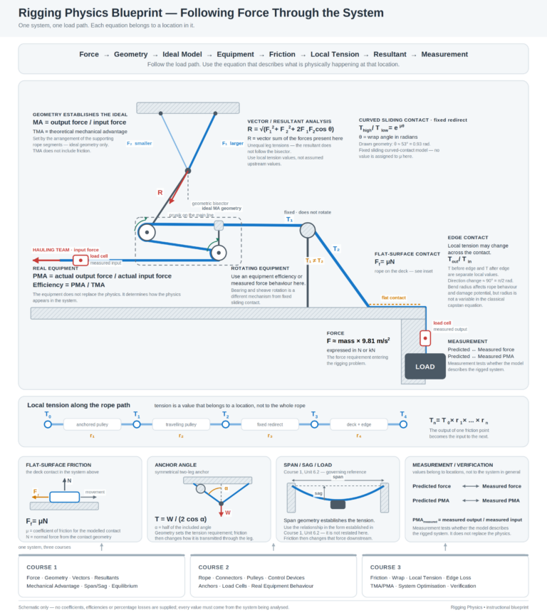
A rope rescue system can be drawn as equipment, but it is better understood as a load path. Force enters the system, geometry establishes how that force should be distributed, equipment turns the ideal arrangement into a physical system, friction changes the force as the rope moves through contact points, and those local tensions eventually become the forces acting at anchors, directionals, and the load. Measurement then gives us a way to compare the system we expected with the one we actually built.
That progression is the backbone of the blueprint:
Force → Geometry → Ideal Model → Equipment → Friction → Local Tension → Resultant → Measurement
The important idea is not the number of equations shown in the graphic. It is that each relationship belongs to a particular location and physical condition in the rigging. Mechanical advantage belongs to the supporting rope geometry. Friction belongs to a contact. Tension belongs to a location along the rope. A resultant belongs where forces actually meet. A load-cell value belongs where the instrument is installed.
Following the load path keeps those relationships connected.
1. Geometry Establishes the Ideal
Before equipment friction, edge contact, or real-world losses are considered, the system needs a reference condition. Geometry provides it.
The arrangement of supporting rope segments establishes theoretical mechanical advantage. Anchor angles establish how applied load is distributed into the legs. Span and sag establish the force conditions in a tensioned system. Vector relationships establish what should happen when two or more forces meet.
This ideal model is not an attempt to pretend friction does not exist. It gives the technician a clean starting point from which the real system can be evaluated.
The unequal-force anchor shown in the blueprint is a good example. The geometric bisector is easy to identify, but the resultant only follows that bisector when the forces entering the point support that condition. Once the leg forces become unequal, the resultant shifts toward the larger force. Geometry still matters, but geometry by itself is no longer the entire answer.
The same principle applies to mechanical advantage. A system may clearly be arranged as a theoretical 3:1, but that describes what the geometry provides. It does not yet tell us what the physical system will deliver.
The ideal model establishes what should happen. The next step is determining what happens when actual equipment is placed into that model.
2. Equipment Turns the Model Into a Real System
The rope path in the main diagram moves through anchored and traveling pulleys before continuing toward a fixed redirect and the edge. At that point, the model is no longer made only of lines and force arrows. Rope, sheaves, bearings, connectors, anchors, and control components are now carrying the load.
That transition matters because real equipment has behavior.
A rotating pulley is intended to change rope direction while allowing the sheave to move with the rope. Its behavior is different from a fixed surface over which the rope must slide. Alignment also becomes important. A pulley that is free to orient with the load path behaves differently from the same pulley trapped against structure or forced into an unfavorable position.
This is where practical mechanical advantage enters the picture. The theoretical ratio still describes the geometry, but the force actually delivered by the physical system depends on how well the equipment transfers that force.
The equipment therefore does not replace the physics established by the ideal model. It determines how that physics appears once the system is built and loaded.
That difference between the ideal and physical system creates the setting in which friction becomes important.
3. Friction Creates Local Tension
The central idea in the blueprint is shown in the strip labeled Local tension along the rope path.
The rope is continuous, but the tension does not automatically remain one universal value from end to end. The force at T₀ belongs to one location. After the rope passes through another part of the system, T₁ belongs to the next location. The same continues through T₂, T₃, and T₄.
Each contact becomes part of that progression.
A rotating pulley has its own equipment losses. A fixed redirect creates a different condition because the rope moves against a surface that does not rotate. A flat contact introduces another friction relationship. At the deck and edge, the rope changes direction while interacting with a structural surface.
These contacts should not be lumped together under a single generic friction percentage. Their physical behavior is different.
What connects them is the sequence. The output from one part of the rope path becomes the input to the next. If a contact changes the tension, the next component receives that changed tension rather than the value that existed farther upstream.
This is why local tension is such an important working concept. It prevents the technician from treating a force calculated or measured in one location as though it automatically exists everywhere else in the system.
Once friction changes the local force, every downstream analysis has to begin with what actually arrives there.
4. What Arrives Downstream Is What Matters
The upper portion of the blueprint brings local tension back into vector and resultant analysis. This is where friction becomes more than a hauling-efficiency issue.
An anchor, master point, or directional responds to the forces that reach it. If one leg arrives carrying more force than another, the resultant reflects that difference. The system does not return to the geometric ideal simply because the legs look symmetrical.
The same is true at the edge. Tension before the edge and tension after the edge are separate local values because the contact lies between them. The edge also introduces rope-bending and damage considerations, so the technician has to distinguish between the force-transfer problem and the physical effect of the bend on the rope.
At the load, the principle becomes even clearer. The load receives what the complete rope path delivers. The theoretical mechanical advantage may still describe the system geometry accurately, but the useful output depends on what happened through the equipment and contacts along the way.
This is why troubleshooting should often move backward through the rope path rather than immediately toward more hardware. If the system does not perform as expected, the cause may be a fixed redirect, edge contact, alignment problem, or other condition that changed the force before it reached the load.
The downstream behavior is frequently the evidence. The cause may be upstream.
5. Measurement Closes the Loop
The blueprint places load cells at the input and output because measurement becomes meaningful once the system has been modeled and the load path understood.
The input measurement tells us what force is being applied at that location. The output measurement tells us what is being delivered at another. Comparing predicted and measured force, or predicted and measured practical mechanical advantage, gives the technician a way to test whether the physical system is behaving as expected.
The location of each measurement is critical. A load cell does not report “the tension in the system.” It reports the force at the point where it is installed.
That makes measurement a verification tool rather than a replacement for system analysis.
If prediction and measurement agree, the model has support under those conditions. If they do not agree, the discrepancy gives the technician a reason to examine the rope path between the relevant locations. The model may have missed a contact, the equipment may be behaving differently than assumed, or the geometry may have changed as the system loaded.
Measurement closes the loop because it connects the ideal model back to the rigging in front of us.
One System, Three Courses
The blueprint also shows how the three Rigging Physics courses connect without becoming three separate subjects.
Course 1 establishes the underlying language of force, geometry, vectors, resultants, mechanical advantage, span, sag, and equilibrium. Course 2 puts rope, connectors, pulleys, control devices, anchors, and load cells into those relationships. Course 3 follows what happens when friction, wrap, edge contact, and real equipment performance change tension from one location to the next.
Together, they produce one working method.
Start with the force. Establish the geometry and the ideal model. Follow that model through the actual equipment. Identify where friction changes the local tension. Use those local forces where they actually arrive. Then measure when the difference between prediction and reality matters.
The system is not understood by knowing one pulley ratio, one equation, or one tension value. It is understood by following the load path and applying the correct relationship to the physical condition that exists at that location.
That is the purpose of the blueprint: one system, one load path, with the physics remaining connected from the initial force all the way through to measured performance.
Peace on your Days
Lance